
19 Feb 2025
In this study, the power dissipation caused by the rotor of a ventilated disc brake was analyzed. Initially, the translational and rotational drag components were described, and subsequently, the main contributing mechanisms due to the weight and inertia of the rotor were highlighted.
As aerodynamics was of primary interest, an in-depth Computational Fluid Dynamics (CFD) simulation of a spinning rotor, while traveling and subjected to a lateral wind, was carried out. The other interacting components, i.e., other brake system parts, wheel, and fork have not been included in the simulation, despite the fact that they would influence the results. The goal of this study was only to gain a preliminary understanding of the aerodynamic properties of the rotor of a disk brake insofar as it increases power dissipation. From an aerodynamic perspective, the front rotor is influenced less by its surroundings and is more comparable aerodynamically to the simulated one. The simulation results pointed out the impacting additional power required to overcome aerodynamic forces and moments, which should be taken into consideration in competitive cycling.
The 16mm diameter rotor chosen for this study is part of the Shimano RT-CL900 ICE TECHNOLOGIES FREEZA and is a good subject because it is a high-performance brake system. It comprises a cooling system with rotating blades designed to dissipate heat by forcing air from its center to the outside metal ring of the rotor.
Major opposing forces to the motion of the cyclist and bicycle system, generated by the rotor are introduced and the following conventions have been used: cyclist and bicycle move at a velocity Vg relative to the ground. Vw is the external wind velocity and ϑ (the crosswind angle) the angle respect to the bicycle direction. The vector sum of Vw and Vg is the relative wind velocity Vr experienced by the cyclist and the angle it forms with the bycicle direction φ is called yaw angle (Figure 1).

The power dissipated by translational aerodynamic drag on the rotor is calculated from its usual definition:
Pt = Ft*Vg
where:
Ft is the translational aerodynamic drag given by Ft = 1/2*Cd*Ar*ρ*Vr2
ρ = air density
Vr = relative wind velocity
Cd = rotor drag coefficient
Ar = relative exposed area of the rotor
Vg = velocity of the cyclist and bicycle relative to the ground.
The rotor is also subject to a rotational moment (respect to its axis of rotation y), My, from the components of drag which are tangential to its rotation, which increases the total power input required to rotate and translate it compared to conditions where only translation is considered. The power dissipated by the rotor's rotational aerodynamic drag is:
Pr = My*ω
where:
My = Fr*r
Fr is the rotational aerodynamic drag given by Fr = 1/2 * Cdr * Ar* ρ * ω² * r²
Cdr = rotor rotational drag coefficient
ω = angular velocity
r = rotor radius.
Power absorbed by the effect of the rotor weight on the rolling resistance of the tire for a bicycle riding on flat ground:
P = Ctire*mr*g*Vg
where:
Ctire is the coefficient of rolling resistance of the tire; it is a function of the tire construction and of the pressure and velocity of the rotation of the wheel.
mr = mass of the rotor.
The contribution of the rotor weight to the rolling resistance in the wheel bearings:
P = Cbear*mr*g*ωb*rb
where:
Cbear is the coefficient of rolling resistance of the bearings, which is a function of the bearing construction.
ωb = ball bearings angular velocity
rb = ball bearing radius.
In the event that the bicycle accelerates, we need to add two more components.
Power is dissipated by the translational acceleration of the center of mass of the rotor:
P = mr*vg*dVg/dt
Power is dissipated by the angular acceleration of the rotor:
P = I*ω*dω/dt
where:
I = moment of inertia of the rotor.
And the following in case of uphill riding:
Power absorbed due to the effect of the rotor weight being lifted uphill with the vertical velocity Vg*sinψ
P = mr*g*Vg*sinψ
where:
ψ inclination of the road.
The model of the rotor was created with a 3D CAD software. The simulation was carried out with OpenFOAM 2312.
The translation velocity Vg of the cyclist and the bike on which the rotor is mounted was set to 14 m/s (50.4 km/h) and the corresponding angular velocity of the rotor is 40 rad/s. The wind velocity Vw was set to 5.1 m/s (18.36 km/h) perpendicular to the direction of motion, ϑ = 90°. The vector sum of external wind Vw and bicycle ground velocity Vg can be used to determine the magnitude of relative wind velocity, Vr , which is 14.9 m/s (53.64 km/h) at a relative yaw angle of ψ = 20°.
The coordinate system was set with the x axis in the opposite direction to the bicycle translation direction, the y axis pointed in the direction lateral to the bicycle, and the z axis pointing up.

In this work, the k-ω SST turbulence model was adopted along with the URANS equations. The simulation was carried out with the PISO (Pressure-Implicit with Splitting of Operators): a pressure-based solver designed for transient simulations of incompressible flow.
To account for the rotation of the rotor, an SM (sliding mesh) method was used. SM utilizes a mesh physical rotation at each time step and is considered highly accurate in the prediction of the flow regimes around rotating rigid bodies. The application of the SM method was carried out using the Arbitrary Mesh Interface (AMI) technique for coupling stationary and rotating mesh regions.
The SM method's success is heavily dependent on the quality of the mesh, the generation of which was a vital part of this work. For the SM method to work correctly, the mesh quality on the interfaces where the rotating and stationary mesh areas meet is especially important. As the boundary region is characterized by steep velocity gradients and intense turbulence, the proper computation of the velocity profile and the turbulent variables in this region was crucial for the accuracy of the numerical solution. A very fine mesh was employed, placing the first cell center at a small distance from the wall (y + < 1), allowing the so-called low-Reynolds number modeling.
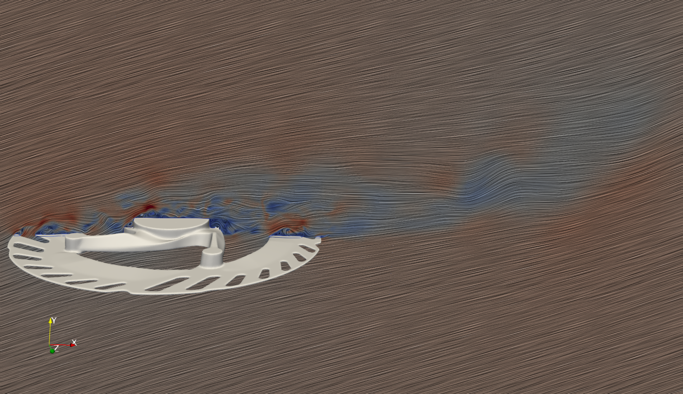
A Line Integral Convolution (LIC) image, with the velocity magnitude color-code, showing a planar slice of the flow perpendicular to the rotor. Vortices formation on the top side of the image are visible.
The CFD simulation output was a opposing drag force Fx = 0.135 N and a resistive rotational moment My = 0.0027 N. These values can be converted in power dissipated by the aerodynamic drag of the rotor:
Px = Fx*Vg = 1.89 W
Pr = My*ω = 0.11 W
Ptot = Px + Pr = 2.00 W
In addition to these forces that oppose motion, the simulation also showed a large value on the side force Fy = 1.35 N, which is 10 times larger than the translational Fx force. Large side forces on an anterior wheel yield strong steering moments and can be a concern of maneuverability.
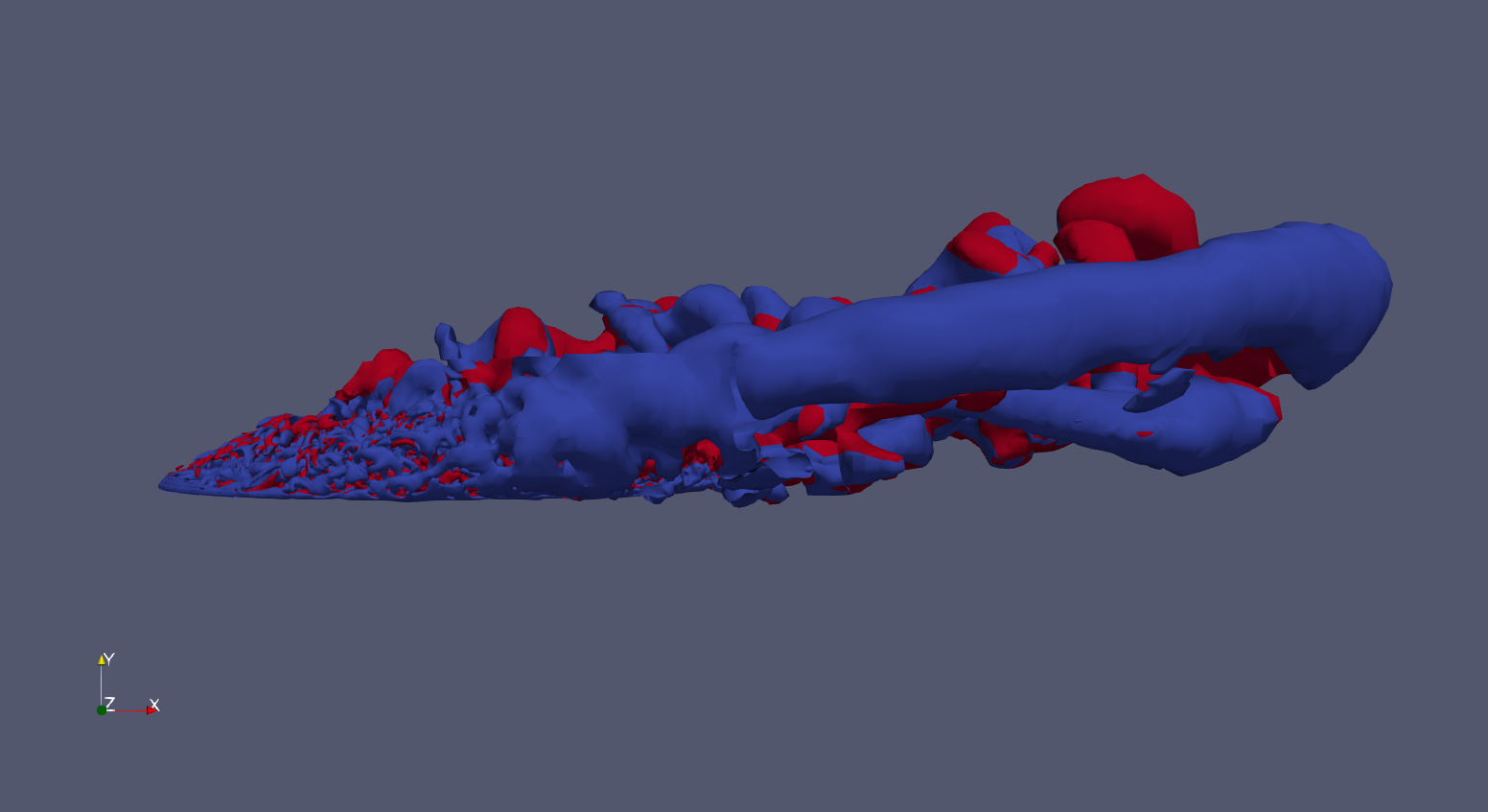
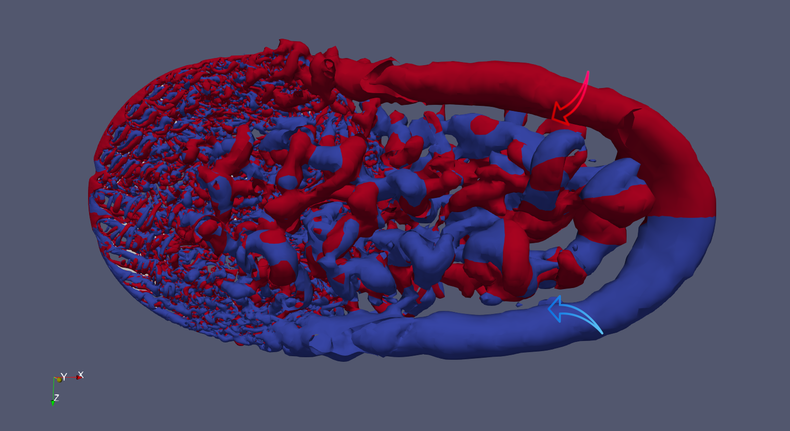
Above, two Q-criterion iso-surface plots colored by vorticity; red is counterclockwise rotation and blue is clockwise rotation. On the left, a top view shows vortices in the relative wind direction. On the right, a side view highlights the primary vortex structures.